Four different dynamical systems

This multimedia post features four different dynamical systems to illustrate some properties of that relevant to my research: we’ll talk about the difference between “integrable” and “chaotic” dynamical systems, and the difference between “continuous-time” and “discrete-time” dynamical systems.


[Some phrases in the text can be expanded for :more info.]

Introduction

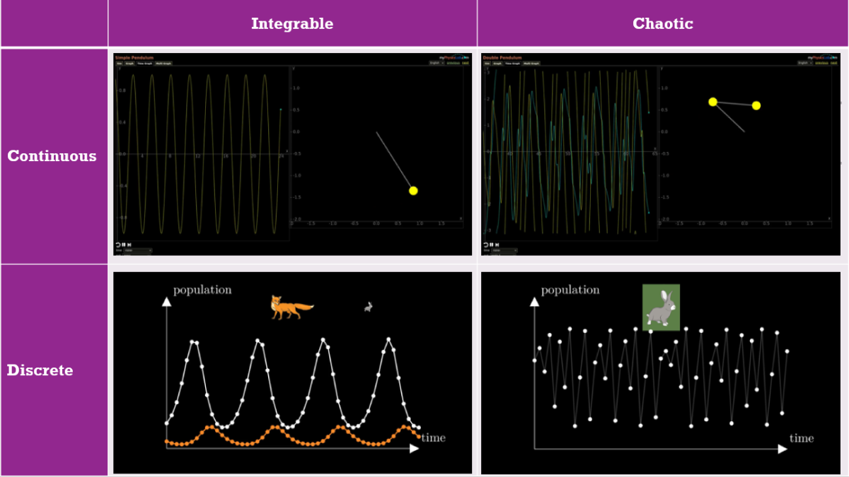
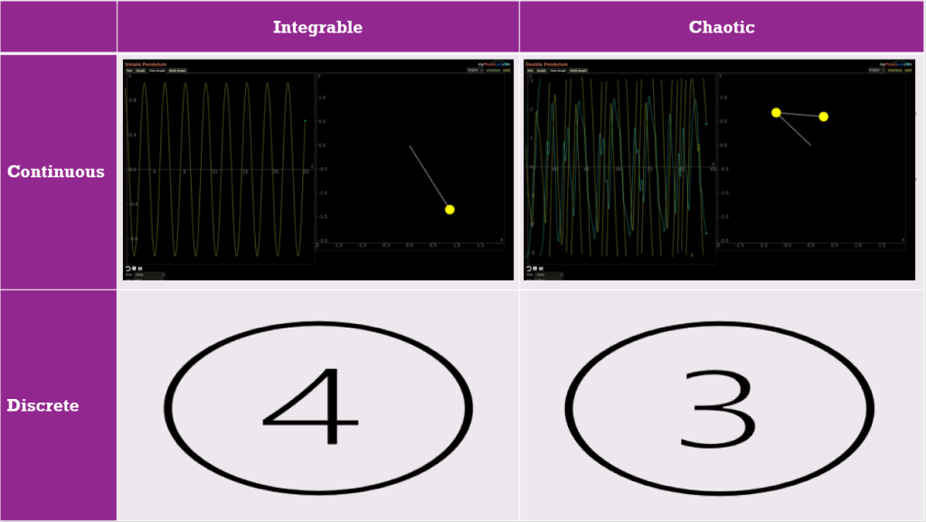
This is an extended write-up of a five-minute talk I gave to an interdisciplinary audience at Loughborough University’s 2022 Research Conference. It features four different :dynamical systems to illustrate some properties of dynamical systems relevant to my research. In particular, we’ll talk about the difference between “integrable” and “chaotic” dynamical systems, and the difference between “continuous-time” and “discrete-time” dynamical systems. So we’ll want to fill up this grid with examples:

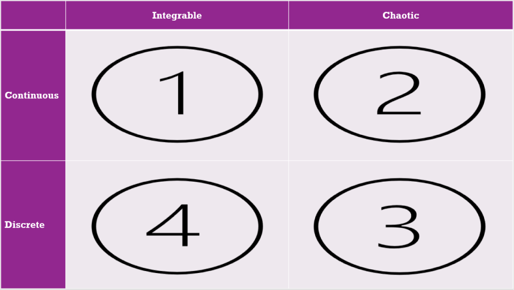
Continuous-time and integrable

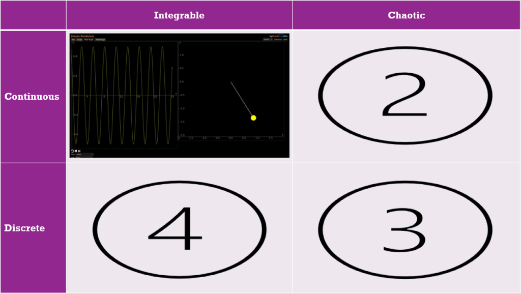
First, let’s consider a :simple pendulum. (Yes, that is the technical term.) This is an object suspended from a string or from a rod that can freely rotate around a hinge. If we give the pendulum a little push, then (ignoring friction) it will keep swinging back and forth again and again.

The graph traced out on the left shows the angle of deflection as a function of time. It is very predictable, and we could write down a formula that precisely describes this graph. The pendulum is an example of an integrable system. “Integrable” is an archaic word for “solvable”: integrable systems are dynamical systems for which we could write down a formula that exactly describes its solution (its state as a function of time). The behaviour of an integrable system is ordered and predictable.

Continuous-time and chaotic

If we attach another pendulum to a simple pendulum, we get a double pendulum. (Yes, that is the technical term.) Let’s give it a good shove and see what happens:

There are now two graphs on the left, representing the angles of both pieces of the pendulum. However, the main difference with the simple pendulum is that these graphs don’t show any repetition or pattern. In fact it is impossible to write down a formula that produces these graphs exactly. Looking at the motion of the system, it is very hard to predict what position it we be in a few seconds into the future. Furthermore, the evolution of the system is :very sensitive to changes in its initial state. These are the properties of a :chaotic system.

You could think of integrable systems and chaotic systems as opposite ends of a wide spectrum representing how dynamical systems can behave.

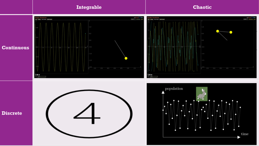
Discrete-time and chaotic

So far, our systems have evolved :continuously in time: they don’t jump instantaneously from a certain state to a completely different one. There are also systems where it doesn’t make sense to keep track of the configuration at every instant. Consider for example a population of animals that breed once per year, at a fixed time of year. To keep track of the population we don’t need to count them every minute of every day. We can just do one count per year at the end of the breeding season. We can then use this count to predict what the population in the next year will be. Such a model is a discrete-time dynamical system: it takes steps in time of a fixed size.

The following model tracks a population of :rabbits living in a certain habitat with limited resources. If the population is small they all have plenty to eat and will produce large litters. If the population is large they compete for resources and will have smaller litters or even die of starvation. We see that the population fluctuates wildly over the years:

These oscillations do not follow a fixed pattern: sometimes the population grows two years in a row, sometimes its goes up and down in alternating years. This makes it very difficult to predict what will happen a few years in the future. So this discrete-time dynamical system is chaotic.

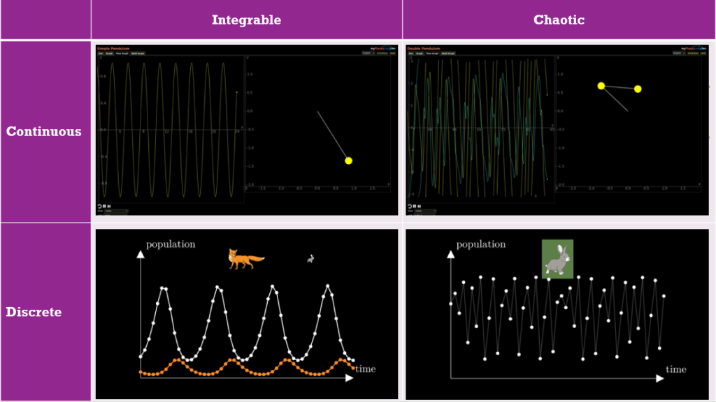
Discrete-time and integrable

In the next :model the rabbits always have plenty to eat, but they are being hunted by foxes.

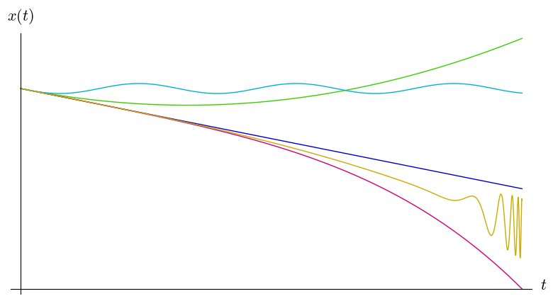
If there are only a few foxes, this does not impact the rabbit population very much and it grows quickly. But then, with many rabbits to eat, the foxes do quite well for themselves. After a few years there are so many foxes that a large proportion of the rabbits gets eaten. The rabbit population declines sharply, leaving the large fox population struggling to find food. This causes the fox population to decline, and the cycle starts over.

In this case the oscillations follow a fixed pattern: the population sizes are predictable and we could theoretically write a formula for the graphs they trace. This discrete-time dynamical system is integrable.

Integrable systems are the exception

The simple pendulum is quite, well, simple. Also the predator-prey model describing our rabbits and foxes is much simpler than any realistic ecological model. There are more complicated integrable systems, but they are relatively rare. If a dynamical system is sufficiently complicated, it is usually chaotic. Integrable systems are the exception. Their nice behaviour and predictabillity is due to some :hidden mathematical structure they possess. This structure can take many different forms. There isn’t one type of hidden structure that explains all integrable systems. Studying all these structures and the relations between them is an active are of research.

Many discrete integrable systems have continuous counterparts, and vice versa. Making the connections between discrete and continuous integrable systems precise often sheds light on their hidden structures. :This approach to studying integrable systems is one of the topics of my research.


:Credits

The first two videos are edited screengrabs from https://www.myphysicslab.com.

The last two videos are my own work [source code] made using Manim and public domain images.

Expandable notes are implemented using :Nutshell.

:x Nutshell

These expandable notes are made using :Nutshell ← Click on the : to expand nested nutshells.

:x D S

The mathematical model of anything that moves or changes is called a dynamical system.

:x T T

Yes, that is the technical term.

:x D P

Three double pendulums with near identical initial conditions diverge over time displaying the chaotic nature of the system. [From Wikipedia]

:x C C

In mathematics, a function is “continuous” if small changes in input lead to small changes in output. In the present context we consider the state of a dynamical system as a function of time, so “continuous” means that if we move forward a very small amount of time, then the change in the system’s state will be correspondingly small.

:x B L B

These rabbits don’t breed like bunnies! They can have large litters, yes, but they only reproduce once per year.

:x L V

This is a discrete-time version of the :Lotka-Volterra model.

:x D S I

For readers with a maths background who want to learn more about discrete integrable systems, I recommend the book Discrete Systems and Integrability by J. Hietarinta, N. Joshi and F. W. Nijhoff.

:x L M S

Readers with a maths background who want find out what some of these structures are, could watch for example the 2020 LMS lecture series Introduction to Integrability.

If you’re after more visual representations on integrable systems, check out What is… an integrable system? where I give a different introduction to integrable systems, using waves as examples.
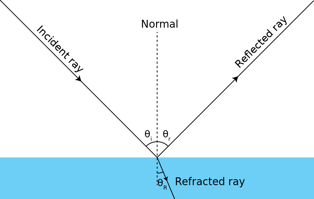
What is… a variational principle?

Variational principles play fundamental role in much of mathematical physics and are a key topic in my own research. That’s a lot to cover, so let’s start with a little story…

Variational principles play fundamental role in much of mathematical physics and are a key topic in my own research. That’s a lot to cover, so let’s start with a little story.

1. An injured cow and the laws of physics

On the morning of a hot summer’s day, a farmer noticed that one of his cows had broken its leg out in the field. The unfortunate the animal would not be able to move for a good while. To make sure the cow wouldn’t get dehydrated, the farmer had to bring it water from the stream bordering the field. While the farmer went to fetch a bucket, he thought about the best way to accomplish this task. What would be the shortest route he could take, that first visits the stream and then goes to the cow?

[Image components by OpenClipart-Vectors and Clker-Free-Vector-Images from Pixabay]

It is fairly obvious that the farmer should take a straight line to the river and then another straight line to the cow. We all learned in school that a straight line is the shortest route between two points. But there are still many ways to combine two straight lines into a suitable path. Which point on the river bank should the farmer go to in order to make the path as short as possible?

If you play around with different possibilities for a minute, you might be able to guess that both lines should make the same angle with the river bank. This simple condition, two angles being equal, is all that is needed to determine the shortest path.

The shortest path to the cow, via the river, consists of two straight lines which are at the same angle to the river bank.

A cow with a broken leg is unfortunate, but it could have been worse. What if the cow had fallen into the river? It won’t be able to get back onto dry land with its leg broken. Luckily the river isn’t too deep, so the clumsy animal won’t drown, but the farmer would have to wade into the river to help it.

Now what would be the fastest way for the farmer to reach the cow? The shortest path would be a straight line, but it is safe to assume that the farmer can run through the field faster than he can wade through the stream. So it’s worth taking a slightly longer path if a shorter part of it is in the water. The quickest route might look like this:

The shortest path is a straight line, but the fastest one has a kink.

The problems our farmer is facing are examples of variational problems. We seek to minimize some quantity (distance or time travelled in these examples). If we have found the optimal solution, then any small variation of this solution will be slightly worse. This gives us a first explanation of the name variational problem.

The cows of physics

Why do we care about these problems? It wouldn’t really make a difference if the farmer takes a few seconds more to reach the cow, would it? And taking a slightly longer route probably wastes less time than overthinking the situation. So what’s all the fuss about?

It turns out that physics is a lot like a farmer trying to help his cow.

As a first example, consider a ray of light reflecting in a mirror. Out of all possible paths from the light source, via the mirror, to wherever the ray of light ends up, it will take the shortest. This is because the law of reflection says that the incident ray and the reflected ray will make the same angle with the mirror. And, as our farmer found out, equal angles create the shortest path.

Or is it the other way around? We might say that the law of reflection holds because light always takes the shortest path.

What about the cow in the river? Well, not just the farmer goes slower in water, so does light. It travels at “light speed” (about 300.000 km/s) in vacuum, marginally slower in air, and a lot slower in materials like water or glass. This matters because I lied to you earlier: light doesn’t necessarily take the shortest path, it takes the fastest path. If the speed of light were the same everywhere, this would make no difference. But if different materials are present, then the speed depends on where you are. So, if, for example, a ray of light enters water from the air, it makes a sudden turn. Just like our farmer did to reach his aquatic cow.

An incoming (“incident”) ray of light can be reflected at the same angle, or refracted at an angle determined by Snell’s law. In both cases, the angle is such that the light reaches its destination as quick as possible. [Image by Nilok at wikimedia commons]

The phenomenon where light changes direction when it enters a different medium is called refraction. You might have learned the formula for the angle of refraction (known as Snell’s law) in your high school physics class:

\(\displaystyle n_i \sin \theta_i = n_R \sin \theta_R.\)


But you don’t need to understand this formula, because it just reflects the fact (no pun intended) that light takes the fastest route. If you want to do calculations, you need formulas. But if you want to understand what’s going on, the variational principle is even better. This particular variational principle, that light always takes the quickest path, is called Fermat’s principle.

As we will see below, light is no exception. Many more physical systems are described by variational principles. They are a cornerstone of every part of modern physics. Like many “laws” of physics, the law of reflection and Snell’s law are nothing but consequences of a simple variational principle.

2. Variational principles in statics

Consider an idyllic landscape of rolling hills…

Photo by Jay Huang, https://flic.kr/p/EDy27K

No, wait. Scratch that! Picture these idealized 1-dimensional rolling hills:

The function U gives the height U(x) of the landscape at position x.

The places where a ball would not immediately start rolling down the hill are those where the tangent line to the hill is horizontal: the tops of the hills and the bottoms of the valleys. In terms of calculus, these are the values of \(x\) where the derivative of \(U\) is zero:

\(\displaystyle \frac{\mathrm{d} U(x)}{\mathrm{d} x} = 0\)

This leads us to a second interpretation of the word variational. The derivative is the infinitesimal rate of change of a function. We can only have a minimum or a maximum if this rate of change, this variation, is zero. Variational problems look for a situation where the infinitesimal variation of some quantity is zero.

In our 1-dimensional landscape, there are eight such locations. There are eight equilibria, where a ball will stay at rest if there is no external force acting on it:

There is a clear difference between the orange balls and the blue balls. The orange ones are on top of hills. Each of them is at a local maximum of the function \(U\). This has the unfortunate consequence that as soon as the ball moves a tiny bit to either side, it will start rolling down the hill, away from its equilibrium. We call these kinds of equilibrium unstable. The blue balls, on the other hand, are at stable equilibria. If a blue ball gets a little kick, it will jiggle about its equilibrium, but eventually it will come back to rest at the same place.

In other words, the variational principle

\(\displaystyle \frac{\mathrm{d} U(x)}{\mathrm{d} x} = 0\)

determines all equilibria, but if we want to make sure we have a stable equilibrium, we need and additional condition. For example, we could require that the second derivative of \(U\) is positive,

\(\displaystyle \frac{\mathrm{d}^2 U(x)}{\mathrm{d}^2 x} > 0.\)

Both conditions combined guarantee that \(U\) has a local minimum at \(x\), or, that the ball will be in a stable equilibrium at position \(x\).

The function \(U\) is called the potential of the system. In this case, where gravity is the only force involved, the potential is essentially the height. In more complex systems, the potential will be a more complicated function of the variables of the system, but its use stays the same. Equilibria are found by applying the variational principle to the potential. Stable equilibria are the local minima of the potential.

3. Variational principles in dynamics

Finding the equilibria of a system is not the whole story. It is good to know where a system can be at rest, but often we also want to understand how it moves when it is not at rest. Miraculously, this is governed by variational principles too.

Suppose we want to keep track of a ball rolling through our 1-dimensional landscape.

We denote the position of the ball at time \(t\) by \(x(t)\). We can make a graph of position over time, so that \(x(t)\) traces out a curve in the \((x,t)\)-plane. Most such curves cannot be realized by a ball moving only under the influence of gravity. Those that can be, are called solutions of the system. For each initial position and velocity of the ball, there will be exactly one solution. But how do we find a solution?

Is any of these curves a solution? How can we tell what kind of graph the position of the ball will trace out?

The most common approach is to use Newton’s second law: Force equals mass times acceleration. In a problem like this, at each location \(x\) the force \(F(x)\) is known. It is determined by the slope of the hill at that position. Acceleration is the second derivative of position with respect to time, so if we know the mass \(m\) of the ball, Newton’s second law gives us the formula

\(\displaystyle \frac{\mathrm{d}^2 x(t)}{\mathrm{d} t^2} = \frac{F(x)}{m}.\)

This is a (second order) differential equation. If the initial position \(x(0)\) and the initial velocity \(\frac{\mathrm{d} x(t)}{\mathrm{d} t} \Big|_{t=0}\) are given, then it can be solved to determine \(x(t)\) for all values of the time \(t\). (At least in theory. Only for relatively simple functions \(F(x)\) will it be possible to write this solution as a nice formula to calculate \(x(t)\).)

Instead of Newton’s second law, we can again use a variational principle. Compared to our previous examples, the quantity we want to minimize is a bit more complicated. Not to worry, though. Once again you don’t need to understand the formula to follow the rest of the text. We want to minimize

\(\displaystyle S[x] = \int_0^T \left( \left( \frac{m}{2} \frac{\mathrm{d} x(t)}{\mathrm{d} t} \right)^2 – U(x(t)) \right)\mathrm{d} t,\)

where the square brackets \([x]\) indicate that \(S\) depends on the function \(x\) as a whole, not just on a particular value \(x(t)\).

We look for minimizers of \(S\) in the following sense. Let the starting position (at time \(0\)) be \(a\) and the final position (at time \(T\)) \(b\), that is \(x(0) = a\) and \(x(T) = b\). Then \(x\) is a solution if \(S[x]\) is smaller than \(S[y]\) for any other function \(y\) with the same boundary values \(y(0) = a\) and \(y(T) = b\).

With some clever calculations, which involve taking variations of the function \(x\), one can see that the functions that minimize \(S\) are exactly those that satisfy Newton’s second law. Once again a famous law of physics turns out to be the consequence of a variational principle.

Variational principles are abundant in physics. I’ve only discussed simple examples here, but it turns out that almost all of modern physics can be formulated using variational principles. In fact the easiest way to describe a physical theory is often to write down the thing it minimizes.

Conserved quantities

The story does not end there. Instead of looking at functions with fixed boundary values to obtain Newton’s second Law, we could look only at functions satisfying Newton’s second law but leave the boundary values unspecified. Then similar “clever calculations” give some information about the boundary values. More specifically, they produce conserved quantities, like the energy of the system, which take the same value at the final time as at the initial time (and indeed at any time in between).

Exactly which conserved quantities come out of this procedure depends on the symmetries of the system. Noether’s theorem, named after early 20th century mathematician Emmy Noether, states that every symmetry corresponds to a conserved quantity. For example, if the system is translation invariant (e.g. billiard balls rolling on a plane) then its total momentum is conserved, and if it is rotationally invariant (e.g. planets orbiting the sun) then the angular momentum is conserved.

Knowing conserved quantities of a system helps to understand its dynamics on many levels. Whether you are looking for an exact solution, a numerical approximation, or a qualitative understanding of the behaviour, conserved quantities will always be of use. And if you have read “What is… an integrable system?“, you know that they are the key to a realm of very peculiar dynamical systems.

5. Sources and further reading

As with many concepts related to physics, a good place to start reading are the Feynman lectures: some relevant chapters are Optics: The Principle of Least Time and The Principle of Least Action.

Even though these physical insights (and the maths) have not changed since the Feynman lectures were published over half a century ago, the cutting edge of science communication has moved on. Nowadays there are excellent educational videos on subjects like this.

Most introductory texts on classical mechanics do not give variational principles the attention they deserve. A notable exception (and excellent book) is

  • Levi, Mark. Classical mechanics with calculus of variations and optimal control: an intuitive introduction. American Mathematical Soc., 2014.

The example of the farmer and the cow is inspired on a problem in

  • Stankova, Zvezdelina, and Tom Rike, eds. A Decade of the Berkeley Math Circle: The American Experience, Volume II. American Mathematical Soc., 2015.

What is… an integrable system?

The oversimplified answer is that integrable systems are equations with a lot of structure. The kind of equations we are thinking about are differential equations, which describe change…

The oversimplified answer is that integrable systems are equations with a lot of structure.

The kind of equations we are thinking about are differential equations, which describe change. Whenever something is moving, you can count on it that physicists would like to describe it using differential equations. It could be an apple falling from a tree or the earth orbiting the sun, the pendulum of a grandfather clock or the waves carrying your phone signal. Here, we’ll look at water waves.

Playing in the water

Let’s start by throwing a pebble in a pond. If you look carefully at the waves it creates, you’ll see some interesting things. You might observe, for example, that longer waves travel faster than shorter waves. After a while you’ll see a sequence of circular waves that are shorter on the inside and longer on the outside:

This effect, that the speed of a wave depends on the wavelength, is called dispersion. The wake of a boat provides another example:

A second effect that you can observe in the videos above is that the individual wave crests and troughs do not travel at the same speed as the big pattern. The velocity of the individual waves is called the phase velocity, the velocity of the whole pattern is called the group velocity.

Phase velocity (red) and group velocity (green). (Source: http://commons.wikimedia.org/wiki/File:Wave_group.gif)

These examples show typical behaviour of waves. The wave fronts change shape and are torn apart. Compared to the ocean on a stormy day, the waves we’ve seen so far are quite tame, but still things get complicated if we try to understand the details.

Integrability

What we saw above is the way most waves work, but they are not integrable systems. Integrable systems are the exceptions. They are differential equations with solutions that are easy to understand. Integrable wave equations describe waves that are really quite boring.

The waves in an integrable system preserve their shape:

Such a wave is called a soliton, because it occurs by itself and (to theoretical physicists) looks like an elementary particle (particle names often end in -on).

Waves in a narrow and shallow channel like in this video are described by the Kortweg-de Vries equation. This equation is one of the most important examples of an integrable wave equation. The understanding of the Korteweg-de Vries equation as an integrable system dates mostly to the 1960s and 70s, but its history started over a century earlier with a Victorian engineer on horseback chasing a soliton along Scottish canal.

Hidden mathematical structure

Unfortunately “having well-behaved solutions” is not a very good mathematical definition of an integrable system. We want to know the underlying reason why certain equations have nice solution. The explanation is usually some hidden structure.

One type of hidden structure that can make a system integrable is the existence of a large amount of conserved quantities. Like its name suggests, a conserved quantity is something that does not change in time. Most systems in physics have conserve quantities like energy and (angular) momentum, but not many more than those. Integrable systems are those that do have a large number of conserved quantities.

In a way, each conserved quantity is an extra constraint that the system must satisfy: the system must always preserve this quantity. So if there are many conserved quantities, then there are many constraints a solution must fulfil. The Kortweg-de Vries equation has an infinite amount of conserved quantities. Therefore, there are infinitely many constraints that the wave must satisfy. This leaves it with little freedom to change its shape. Initially there might still be some complicated things going on, with smaller waves behaving erratically, but once a large stable wave is formed, it will keep its shape forever.

Conserved quantities are not only part of the explanation of the nice qualitative behaviour we observed, they also help to make quantitative statements about a system. Knowing conserved quantities is very helpful to derive exact solutions of a differential equation. An exact solution is a formula that tells you precisely which shape and position the wave takes at each instant in time. Nowadays we call finding exact solutions “solving” a differential equation, but in the 19th century people would say “integrating” instead. This is where the name integrable system comes from.

Soliton interaction

When two solitons collide, weird stuff happens. Their interaction is complicated and looks a bit chaotic. You’d expect the combined wave to be taller, but actually the height of the crest decreases during the interaction.

But then, magic! After the interaction, the two original waves appear again, as if nothing at all has happened! Even though the waves seem to change during the interaction, the integrable system “remembers” everything about them and in the end they are restored.

One sentence about my work

My research involves a relatively new approach to integrable systems, which is to describe them using variational principles.

You can find out here what a variational principle is. Or, if you’ve had enough maths for one day, you can head to Gloucestershire instead and try to surf a soliton:

You can find a more technical introduction
to integrable systems in these slides